Quantitative Trading: example 3.6 Pairs trading with GLD and GDX
This example illustrates how to separate the data into a training set and a test set.
We will backtest a pair-trading strategy and optimize its parameters on the training set and look at the effect on the test set. GLD versus GDX is a good candidate for pair trading because GLD reflects the spot price of gold, and GDX is a basket of gold-mining stocks. It makes intuitive sense that their prices should move in tandem.
E. Chan states that he has discussed this pair of ETFs extensively on his blog in connection with cointegration analysis (see, e.g., epchan.blogspot.com/2006/11/reader-suggested-possible-trading.html).
Cointegration analysis on the training set is covered in Chapter 7 of the book and is used to determine if the spread formed by long GLD and short GDX is mean reverting. In this example we will perform a regression analysis on the training set to determine the hedge ratio between GLD and GDX, and then define entry and exit thresholds for a pair-trading strategy. We will see how optimising these thresholds on the training set changes the performance on the test set.
We will use a function, lag1, to lag the time series by one time period.
# make sure previously defined variables are erased.
rm(list = ls())
library(pracma)
library(echanFuncs)
library(matlab)
library(dplyr)
# read a spreadsheet named "GLD.xls" into MATLAB.
gld_in <- read.csv(file.path("data", "GLD.csv"))

# the first column (starting from the second row) is the trading days in
# format mm/dd/yyyy.
tday_gld <- gld_in$Date

# convert the format into yyyymmdd.
tday_gld <- format(as.Date(tday_gld, "%d/%m/%Y"), "%Y%m%d")

# convert the date strings first into cell arrays and then into numeric format.
tday_gld <- as.numeric(as.character(tday_gld))

# the last column contains the adjusted close prices.
cls_gld <- gld_in$Adj.Close

# date and adjusted close as data.frame
gld_dat <- data.frame(tday = tday_gld,
                      cls_gld = cls_gld)

# read a spreadsheet named "GDX.xls" into MATLAB.
gdx_in <- read.csv(file.path("data", "GDX.csv"))

# the first column (starting from the second row) is the trading days in
# format mm/dd/yyyy.
tday_gdx <- gdx_in$Date

# convert the format into yyyymmdd.
tday_gdx <- format(as.Date(tday_gdx, "%d/%m/%Y"), "%Y%m%d")

# convert the date strings first into cell arrays and then into numeric format.
tday_gdx <- as.numeric(as.character(tday_gdx))

# the last column contains the adjusted close prices.
cls_gdx <- gdx_in$Adj.Close

# dataframe of the data
gdx_dat <- data.frame(tday = tday_gdx,
                   cls_gdx = cls_gdx)

# find the intersection of the two data sets, and sort them in ascending order
# by the time
all_dat <- left_join(gdx_dat, gld_dat, by = "tday")
all_dat <- all_dat[order(all_dat$tday),]

# define indices for training set
trainset <- 1:252

# define indices for test set
testset <- seq(length(trainset)+1, nrow(all_dat), 1)

# determines the hedge ratio on the trainset
# use regression function
results <- lm(I(all_dat[trainset, "cls_gld"])~0+all_dat[trainset, "cls_gdx"])

hedgeRatio <- results$coefficients[[1]]
hedgeRatio
## [1] 1.631009
# spread = GLD - hedgeRatio*GDX
spread <- all_dat[, "cls_gld"] - hedgeRatio*all_dat[, "cls_gdx"]
plot(spread[trainset])

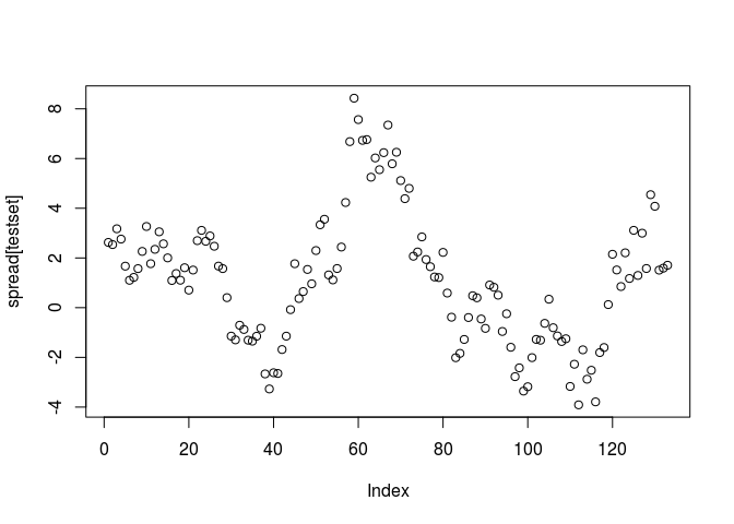
plot(spread[testset])
# mean  of spread on trainset
spreadMean <- mean(spread[trainset])

# standard deviation of spread on trainset
spreadStd <- sd(spread[trainset])

# z-score of spread
zscore <- (spread - spreadMean) / spreadStd

# buy spread when its value drops below 2 standard deviations.
longs <- zscore <= -2

# short spread when its value rises above 2 standard deviations.
shorts <-  zscore >= 2

# exit any spread position when its value is within 1 standard deviation of
# its mean.
exits <- abs(zscore) <= 1

# initialize positions array
# positions=NaN(length(tday), 2)
positions <- matrix(rep(NaN), nrow(all_dat), 2)

# long entries
positions[shorts, ] <- repmat(c(-1, 1), sum(shorts), 1)

# short entries
positions[longs, ] <- repmat(c(1, -1), sum(longs),  1)


# exit positions
positions[exits, ] <- matlab::zeros(length(find(exits)), 2)

# ensure existing positions are carried forward unless there is an exit signal
positions <- fill_missing_data(positions)

# combine the 2 price series
cl <- data.frame(cls_gl = as.numeric(all_dat$cls_gl),
                 cls_gdx = as.numeric(all_dat$cls_gdx))

# Original MATLAB: dailyret=(cl - lag1(cl))./lag1(cl)
lag1_cl <- lag1(cl)
## [1] "is numeric"
lag1_cl <- data.frame(cls_gl = as.numeric(lag1_cl$cls_gl),
                      cls_gdx = as.numeric(lag1_cl$cls_gdx))


dr_1 <- cl[2:nrow(cl), ] - lag1_cl[2:nrow(lag1_cl), ]

dailyret <- rbind(lag1_cl[1, ], dr_1 / lag1_cl[2:nrow(lag1_cl), ])

# MATLAB original: pnl=sum(lag1(positions).*dailyret, 2)
pnl <- rowSums(lag1(positions)[2:nrow(positions), ]*
                      dailyret[2:nrow(dailyret), ])
## [1] "is numeric"
pnl <- c(NA, pnl)

# the Sharpe ratio on the training set should be about 2.3
sharpeTrainset <- sqrt(252) *
  mean(pnl[trainset[2:length(trainset)]]) / sd(pnl[trainset[2:length(trainset)]])
sharpeTrainset
## [1] 2.327844
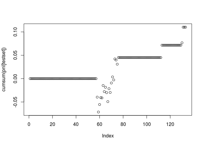
# the Sharpe ratio on the test set should be about 1.5
sharpeTestset=sqrt(252) * mean(pnl[testset], na.rm = TRUE) / sd(pnl[testset])
sharpeTestset
## [1] 1.508212
plot(cumsum(pnl[testset]))